Climate Toolbox

Hi!
My name is Maria Chara Karypidou and I am a PhD candidate in Climatology.
I am located at the Department of Meteorology and Climatology, at the Aristotle University of Thessaloniki, in Greece.
This tiny dot of the internet is my attempt to communicate bits of code with some functionality in climate sciences. This is a work in progress and more chapters and sub-chapters will be added gradually.

For any comment, correction or tutorial suggestion please contact me at: karypidou@geo.auth.gr

Dynamics of the Atmosphere

More coming soon...

Relative Vorticity

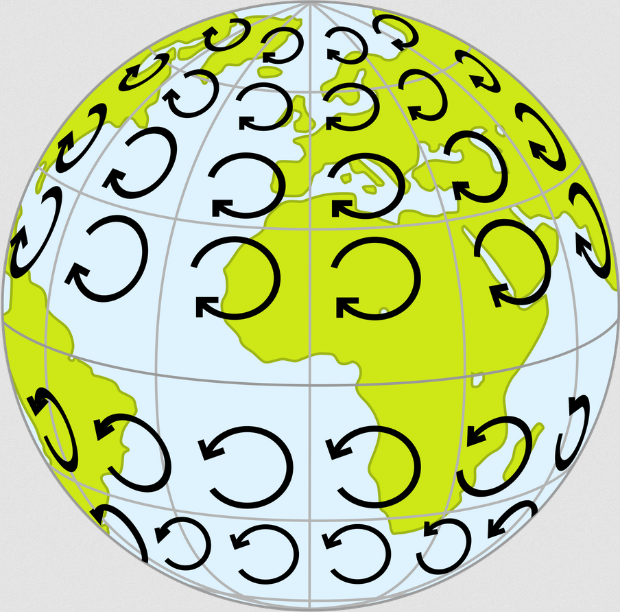
In a way, wind is in a continuous dance mode around the globe. Nonetheless, it is also performing a local dance, spinning around itself. In dynamic meteorology, this movement of the wind is described by a quantity termed as "relative vorticity". Briefly, relative vorticity is a measure of the spin of an air mass.

First Thoughts

Relative vorticity is an invaluable variable for meteorologists and climatologists. It can be very "noisy" at the lower troposphere (850 hPa), but it can provide very indicative information about atmospheric disturbances at the middle or higher troposphere (250 hPa).

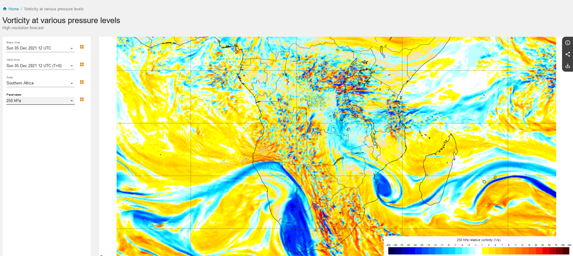
Relative vorticity at 250 hPa from the ECMWF forecasting system for 6 December 2021 at 12.00 UTC over southern Africa.

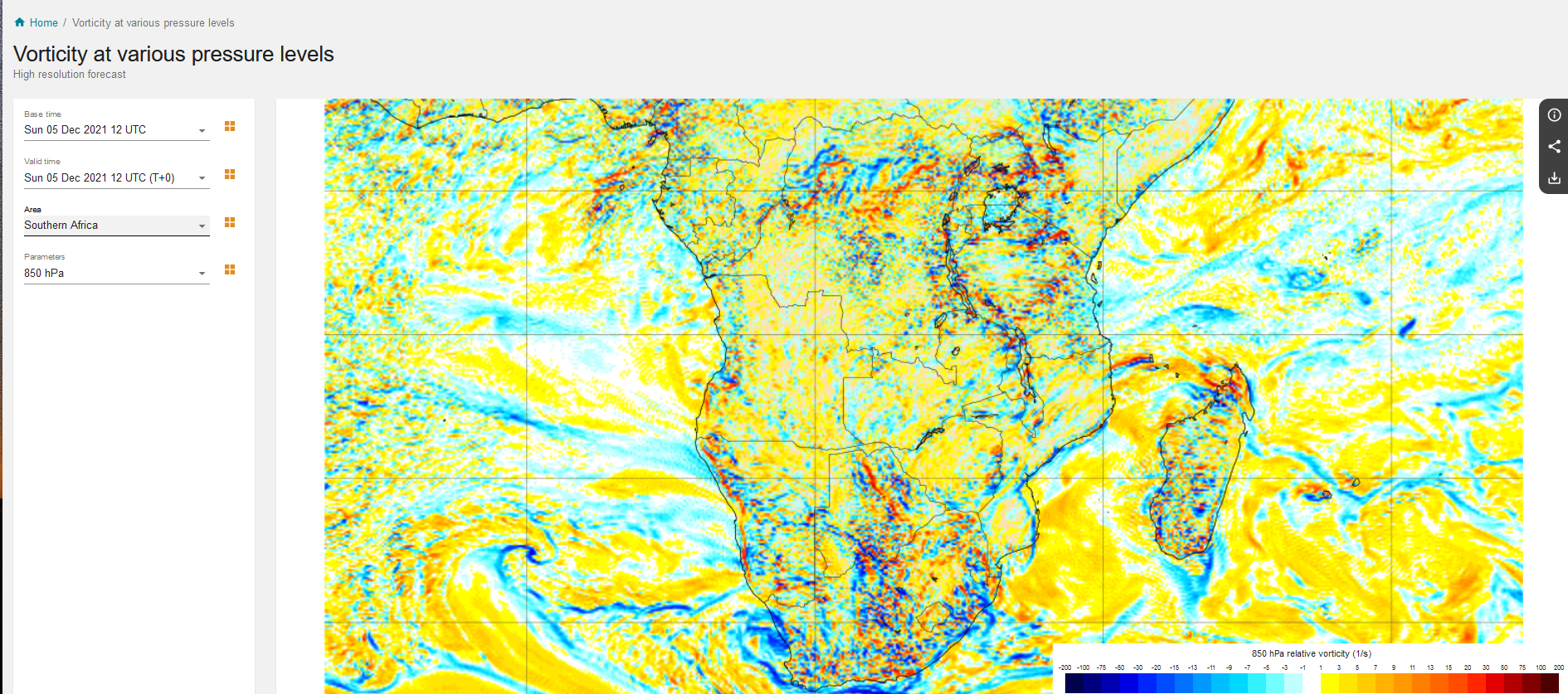
Relative vorticity at 850 hPa from the ECMWF forecasting system for 6 December 2021 at 12.00 UTC over southern Africa.

Theory

Theory is taken from the book "An Introduction to Dynamic Meteorology" by James R. Holton and Gregory J. Hakim.

According to them, "Vorticity, the microscopic measure of rotation in a fluid, is a vector field defined as the curl of velocity. The relative vorticity $\omega$ is the curl of the relative velocity":

$\omega \equiv \nabla\times \U$

which, in Cartesian coordinates, is analyzed to the following:

$\omega = (\frac{\partial w}{\partial y} - \frac{\partial v}{\partial z}, \frac{\partial u}{\partial z} - \frac{\partial w}{\partial x}, \frac{\partial v}{\partial x} - \frac{\partial u}{\partial y})$

After performing scale analysis on the above equation, it appears that the horizontal components are negligible, and therefore only the vertical component is used, leading to the following equation for relative vorticity:

$\zeta = \frac{\partial v}{\partial x} - \frac{\partial u}{\partial y}$

Code

This tutorial is based on the MetPy Python library and exploits the vorticity function.
Before using the vorticity function, let's take a look at the code. MetPy's repository is openly accesible in Github, making our lives easier. If we move to the source code of the Kinematics directory and look within lines 26-67, we will have a closer look of what happens within the function.

def vorticity(u, v, *, dx=None, dy=None, x_dim=-1, y_dim=-2):
    r"""Calculate the vertical vorticity of the horizontal wind.

As we see, the vorticity function requires the U and V wind components as input. In addition, some information about the dx and dy is required, referring to the grid spacing on the Y and the x-axis.

dudy = first_derivative(u, delta=dy, axis=y_dim)
dvdx = first_derivative(v, delta=dx, axis=x_dim)
return dvdx - dudy

The key information is provided in lines 65-57. As we see, finite differences are calculated using the first_derivative function. The first_derivative function uses forward and backward differencing at the edges of the domain and central differences at every other part of the domain. We are reminded that in first order finite differencing, the following formulas are applied:

The one-sided (forward) difference: $\frac{f(a \dotplus h)-f(a)}{h}$
The one-sided (backward) difference: $\frac{f(a)-f(a-h)}{h}$
The central difference: $\frac{f(a \dotplus h)-f(a-h)}{2h}$

The partial derivatives are then subtracted using the formula: $\frac{\partial v}{\partial x} - \frac{\partial u}{\partial y}$

Hands-on

For this exercise we use the ERA5 function reanalysis dataset, downloaded from the Copernicus Climate Data Store. For the calculation of relative vorticity we will need the U and V wind components. The region of interest is southern Africa and extends between latitudes from -10 to -35 oS and between longitudes from 10 to 42 oE. Using the following command in a linux environment, we can see some attributes of the file we use and what preprocessing has taken place.

ncdump -h ERA5_daymean_monmean_merge_800.nc

We see the following:

dimensions:
        time = UNLIMITED ; // (240 currently)
        bnds = 2 ;
        longitude = 129 ;
        latitude = 101 ;
variables:
        double time(time) ;
                time:standard_name = "time" ;
                time:long_name = "time" ;
                time:bounds = "time_bnds" ;
                time:units = "hours since 1900-01-01 00:00:00.0" ;
                time:calendar = "gregorian" ;
                time:axis = "T" ;
        double time_bnds(time, bnds) ;
        float longitude(longitude) ;
                longitude:standard_name = "longitude" ;
                longitude:long_name = "longitude" ;
                longitude:units = "degrees_east" ;
                longitude:axis = "X" ;
        float latitude(latitude) ;
                latitude:standard_name = "latitude" ;
                latitude:long_name = "latitude" ;
                latitude:units = "degrees_north" ;
                latitude:axis = "Y" ;
        double u(time, latitude, longitude) ;
                u:standard_name = "eastward_wind" ;
                u:long_name = "U component of wind" ;
                u:units = "m s**-1" ;
                u:_FillValue = -32767. ;
                u:missing_value = -32767. ;
        double v(time, latitude, longitude) ;
                v:standard_name = "northward_wind" ;
                v:long_name = "V component of wind" ;
                v:units = "m s**-1" ;
                v:_FillValue = -32767. ;
                v:missing_value = -32767. ;

// global attributes:
                :CDI = "Climate Data Interface version 1.9.7.1 (http://mpimet.mpg.de/cdi)" ;
                :Conventions = "CF-1.6" ;
                :history = "Thu Nov 04 17:29:33 2021: cdo merge ERA5_u800_1986_2005_regionA_daymean_monmean.nc ERA5_v800_1986_2005_regionA_daymean_monmean.nc ERA5_daymean_monmean_merge_800.nc\n",
                        "Thu Nov 04 17:17:03 2021: cdo monmean ERA5_u800_1986_2005_regionA_daymean.nc ERA5_u800_1986_2005_regionA_daymean_monmean.nc\n",
                        "Thu Nov 04 17:13:32 2021: cdo daymean ERA5_u800_1986_2005_regionA.nc ERA5_u800_1986_2005_regionA_daymean.nc\n",
                        "Sun Oct 31 16:42:02 2021: cdo sellonlatbox,10,42,-35,-10 ERA5_u800_1986_2005.nc ERA5_u800_1986_2005_regionA.nc\n",
                        "Sun Oct 31 16:12:56 2021: cdo -b F64 -f nc2 mergetime ERA5_u800_1986_1998.nc ERA5_u800_1999_2005.nc ERA5_u800_1986_2005.nc\n",
                        "2021-10-31 03:41:27 GMT by grib_to_netcdf-2.23.0: /opt/ecmwf/mars-client/bin/grib_to_netcdf -S param -o /cache/data9/adaptor.mars.internal-1635647195.7786794-18405-5-3a45d373-0572-4b14-8ed9-085c098ef857.nc /cache/tmp/3a45d373-0572-4b14-8ed9-085c098ef857-adaptor.mars.internal-1635638913.5616663-18405-6-tmp.grib" ;
                :frequency = "mon" ;
                :CDO = "Climate Data Operators version 1.9.7.1 (http://mpimet.mpg.de/cdo)" ;
}

The file contains mean monthly data from 1986-2005 of U and V wind components at 800hPa (240 timesteps in total).

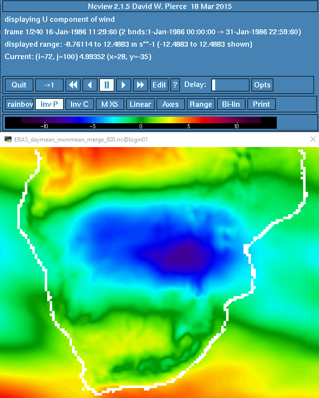
ERA5 data over southern Africa. Map displays the first timestep 1986/01 of the U-Wind component.

So, moving to the python code, we first have to load all packages and functions we will use.

# 
from matplotlib import pyplot
from matplotlib.cm import get_cmap
from __future__ import print_function
from netCDF4 import Dataset,num2date,date2num
from matplotlib.colors import from_levels_and_colors
from cartopy import crs
from cartopy.feature import NaturalEarthFeature, COLORS
from metpy.units import units
from datetime import datetime
from metpy.plots import StationPlot
#
import metpy.calc as mpcalc
import xarray as xr
import cartopy.crs as ccrs
import matplotlib
import numpy as np
import matplotlib.pyplot as plt
import cartopy.feature as cfeature
#

We continue by setting our path:

root_dir = '/my/.../path/.../'

And load in our NetCDF file:

nc = Dataset(root_dir+'ERA5_daymean_monmean_merge_850.nc')

We then extract the longitude (lon) and latitude (lat) variables from our NetCDF file for later use.

lon=nc.variables['longitude'][:]
lat=nc.variables['latitude'][:]

As we saw in the Code section, the vorticity function requires some information about the grid spacing of the NetCDF file we use. We provide this information through the lat_lon_grid_deltas command.

dx, dy = mpcalc.lat_lon_grid_deltas(lon, lat)

Also, in the attributes of the NetCDF we saw that the file contains 240 timesteps (monthly values from 1986-2005). Therefore, we can perform our calculations 240 times or more wisely, apply a loop.

#
u = []
v = []
vort = []
#
for i in range(240):
    v.append(np.array(nc.variables['v'][i,:,:]))                    
    u.append(np.array(nc.variables['u'][i,:,:]))
    v[i] = units.Quantity(v[i], 'm/s')
    u[i] = units.Quantity(u[i], 'm/s')
    vort.append(np.array(mpcalc.vorticity(u[i], v[i], dx=dx, dy=dy)))
    #
    print(i)
#

Checking the dimensions of our "vort" object, we see that it has 240 timesteps, 129 longitude and 101 latitude values.

np.shape(vort)

And now comes the plotting time!

min_val = np.min(vort)
max_val = np.max(vort)
#
dataproj = ccrs.PlateCarree()
#
# Set the figure size, projection, and extent
fig = plt.figure(figsize=(2.7,2.8))
ax = plt.axes(projection=ccrs.Robinson())
ax.coastlines(resolution="110m",linewidth=1)
ax.gridlines(linestyle='--',color='black')
#
# Set contour levels, then draw the plot and a colorbar
clevs = np.arange(-0.0001,0.0001,0.000011)
plt.contourf(lon, lat, vort[0], clevs, transform=ccrs.PlateCarree(), cmap=get_cmap("bwr"), extend="both")
#
cb = plt.colorbar(ax=ax, orientation="vertical", pad=0.002, aspect=16, shrink=0.8)
cb.set_label(size=6, rotation=270, labelpad=15, label='[s$^{-1}$]')
cb.ax.tick_params(labelsize=4)
#
fig.savefig('ERA5_vort_tutorial_1-1-1986.png', format='png', dpi=300)
#

The resulting map is displayed below. All negative values indicate cyclonic relative vorticity (remember that we are in the southern hemisphere) and all positive values display anticyclonic relative vorticity.

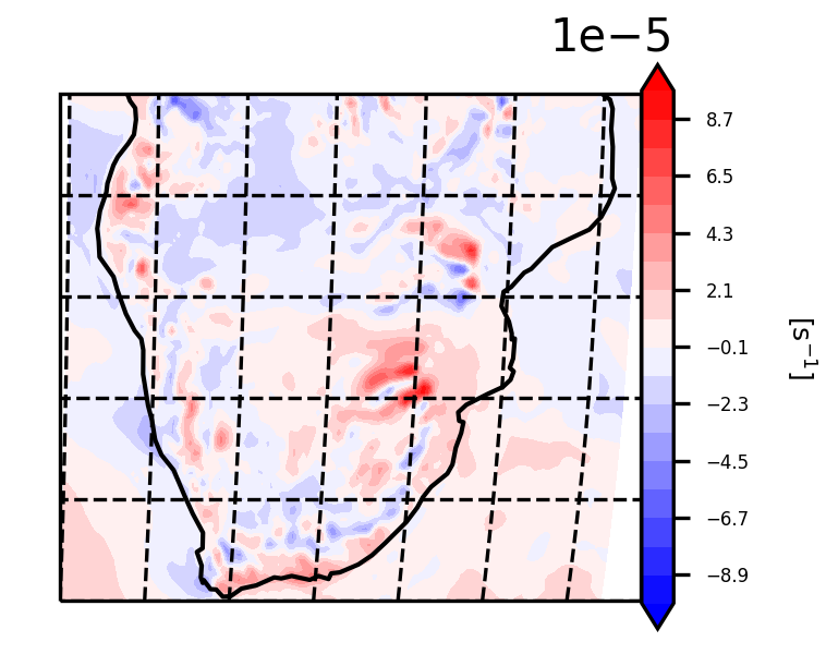
Relative vorticity at 800 hPa for 1986/01 constructed using U and V wind components from ERA5 reanalysis data over southern Africa.

Absolute Vorticity

As discussed in the previous section, the localised spin of an air mass is described by a quantity termed "Relative Vorticity". However, as the earth rotates, it is also having an impact on the motion of air masses.

Vorticity Advection

Thermodynamics of the Atmosphere

ClimateToolbox: Hands-on Theory and Code

Climate Toolbox

Dynamics of the Atmosphere

Relative Vorticity

First Thoughts

Theory

Code

Hands-on

Absolute Vorticity

First Thoughts

Theory

Code

Vorticity Advection

First Thoughts

Theory

Code

Thermodynamics of the Atmosphere

Potential Temperature